Dec 14, 2017 | Developer | Report | Source code

Computational PhotographyMatlab

Overview

Our project is based on Hays et al. 2008 paper Scene Completion Using Millions of Photographs. In this project, an image database with more than four hundred thousand photos will be set up, and the algorithm will be able to patch up the holes of an input image with images both structurally and semantically similar.

Database Setup

We use Flicker API to download large sets of images online. We select several categories of images based on keywords such as Chicago and lake. Since Flicker API limit is to return only 400 images per API request, we handle this issue by making multiple API calls according to the date the images were uploaded. During the downloading process, we notice that with such a large amount of data, it takes more than half a month to download all the images. To boost the download speed, we design and implement a multithread downloader in Python. Also, to avoid having invalid or useless images, we prune out all the photos smaller than 800 * 600 px or have an edge larger than 10000 px. Finally, we managed to download around 450,000 images in parallel within 30 hours and used these images as the pool for image completion.

After setting up a large image database, our algorithm will first select the best semantically matching scenes and perform traditional template matching.

Semantic Structure Matching

To implement a perfect image completion and avoid the long searching time, we need to find a group of candidate images that match the scenes in input image semantically. To find semantically similar images, we used the GIST descriptor to model the images. GIST descriptor is described in Oliva et al. 2001 paper Modeling the shape of the scene: a holistic representation of the spatial envelope. GIST is a low-dimensional representation of an image, where some perceptual dimensions such as openness, roughness and expansion are considered. Images with scenes in the same categories will get close GIST descriptors.

We use a Python library called Lear GIST python, which implements the GIST descriptor in the paper.

First, we calculate the GIST descriptor for every image using a multiprocess algorithm in our image database and store all in .npy files for fast reading and writing.

Second, we calculate a weighted GIST descriptor for the to-be-filled image with its mask for the hole. The GIST is weighted by the proportion of valid pixels (not in the hole) in every spatial bin.

Finally, we calculate the L1 distance between the GIST for the input image and the GIST for images in the database. We also calculate the SSD (Sum of Square Distance) between the input image and images in the database. Then we assign weights to these two attributes and pick 20 images that have the smallest values as input images for the next step.

Local Context Matching

We now have 20 semantically nearest scenes, and we can use our local template matching algorithms to find the best matches. We further divide the steps into two: Seam Finding and Poisson Blending, inspired by previous Project 2 and Project 3.

We iterate the following process on each selected image:

Setup Input Image

When the program starts, we can manually select the area to erase or input the incomplete image and its mask.

Cut Seam Finding

To find the minimum-cost path around the irregular border, we first find the smallest rectangle containing the irregular hole, then add 80 to each of the four edges to get a larger rectangle as well and minus 80 to each border, to get a smaller rectangle. We regard the difference between the large and small rectangles (the width of the border is 160 in our case) as local context, i.e., the overlapping region of the existing and sampled patch.

Note that the blue rectangle is the smallest rectangle containing the irregular hole. We perform the graph cut between the yellow rectangle and the orange rectangle.

Take the top 160 * width region as an example. We use the idea of buildErrpatch in Project 2, but add some modifications to satisfy the need of irregular shape. First, we calculate the SSD of two images on L*a*b color space instead of RGB color space. Since the region we need to cut contains part of the holes, we changed the overlap region of the hole and cut to Inf so that it won’t be marked as the cut edge. Then, we use cut to find the minimum cost path from the left to the right side of the patch, which defines a binary mask for the whole local context region.

We apply the above process to all four edges (top, bottom, left, right). Note that to find the cut for the left and right region, we need to transpose the region first so that we can find the cutting path from top to bottom side in the original region. We store the minimum cost for each time, and let the sum be the total cut cost. Find the intersection of four masks.

Poisson Blending

After we get the mask, we use the standard poissonBlend by Project 3 on the whole image region to compose the image.

Note that different from Project 3 which allows the user to select mask region, our mask is computed by the cut, so there might be isolated pixels or regions with weird border. Since Poisson Blending is based in neighboring regions, before outputting mask in the process above, we smooth the mask a little bit.

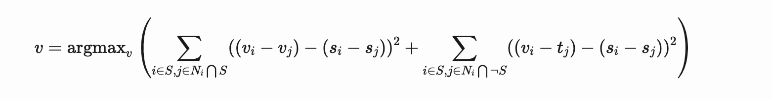
We use the Poisson Blending formula to solve blending constraints.

Calculate Costs and Ranks

To calculate costs, we add up three scores: GIST distance, graph cut cost, and Poisson blending cost. After writing 20 output images, storing costs and ranking from smallest to largest, we select the top 5 matches.

No.1 2005_10_13_31.jpg: gistdist=0.072752 cutcost=8.921728   blendcost=1.555726
No.2 2005_10_3_33.jpg:  gistdist=0.056394 cutcost=140.355418 blendcost=8.606997
No.3 2005_11_14_38.jpg: gistdist=0.039884 cutcost=35.207486  blendcost=3.811644
No.4 2005_11_38_49.jpg: gistdist=0.085163 cutcost=7.682632   blendcost=2.521401
No.5 2005_1_4_33.jpg:   gistdist=0.092792 cutcost=356.132497 blendcost=6.827347

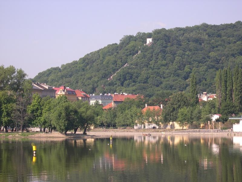
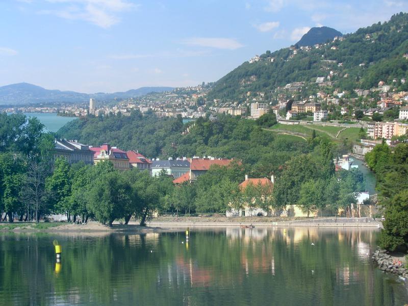
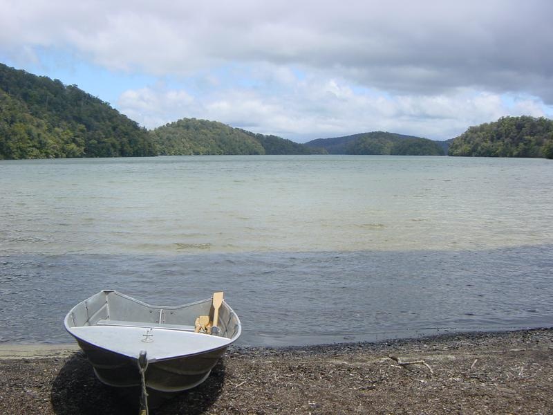
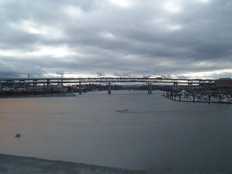
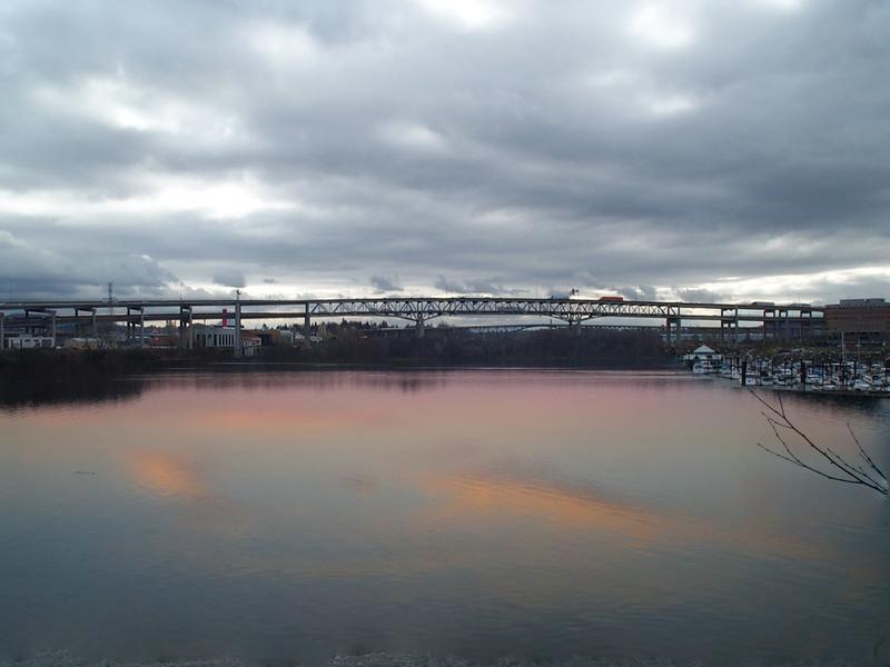
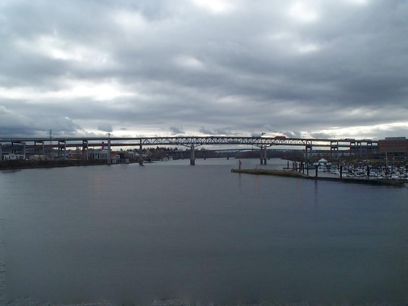
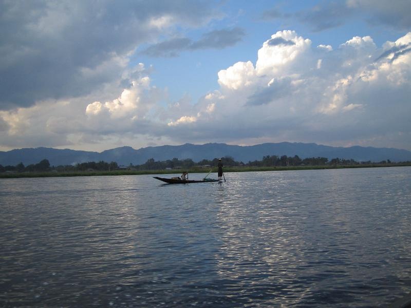
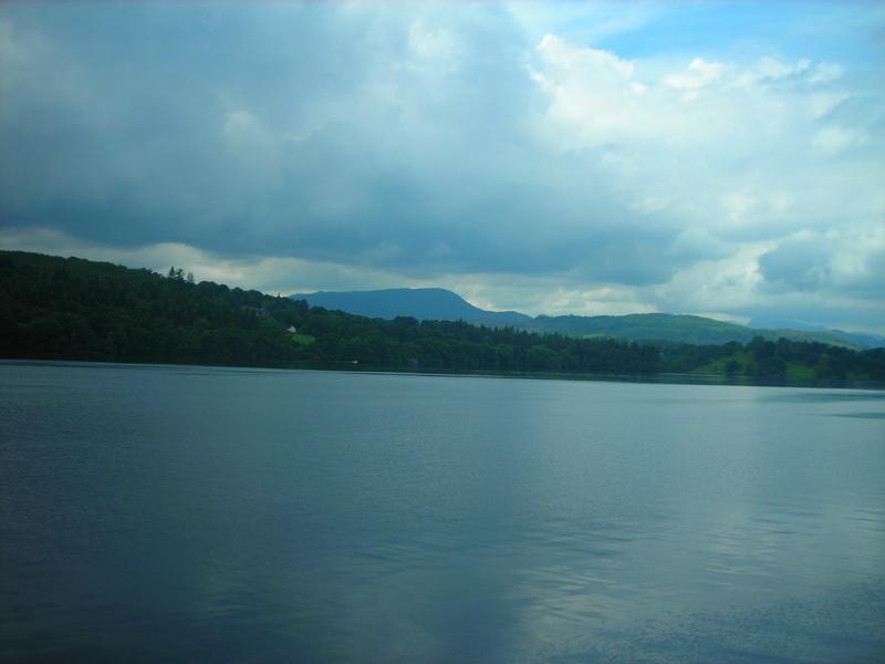
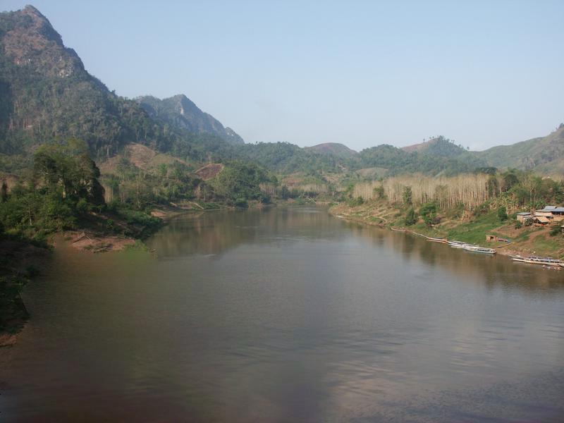
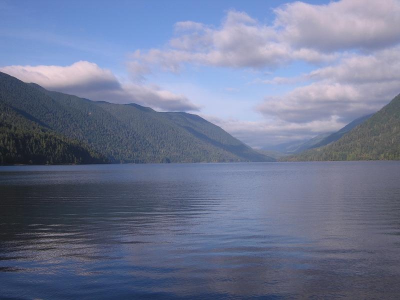
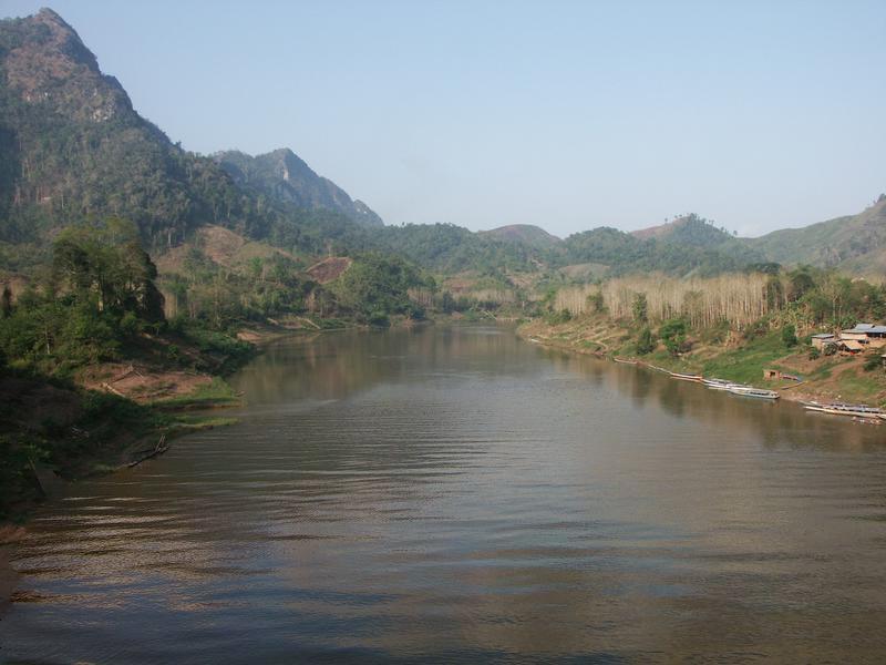
Results

For better display, see our project page.

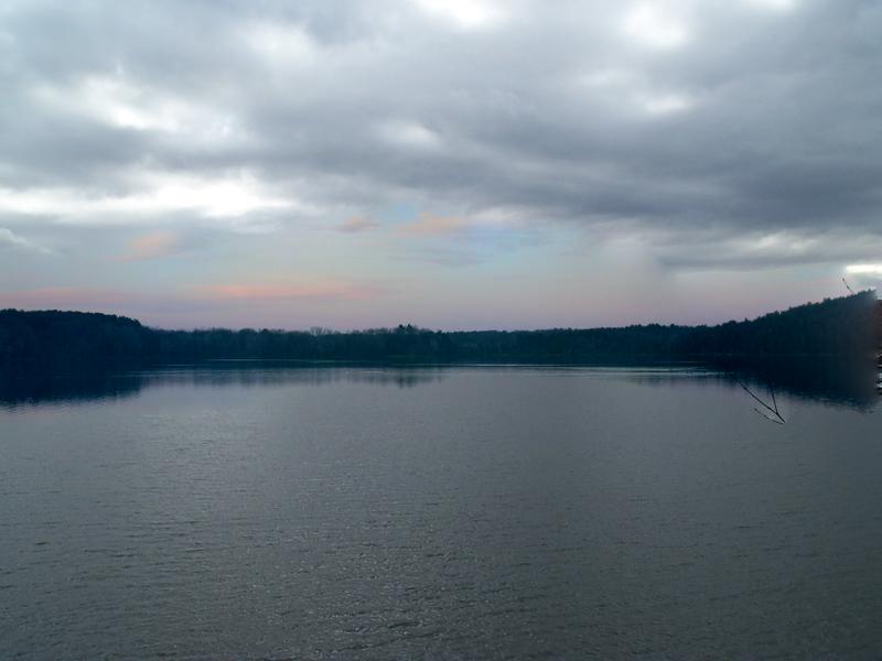
Test Result 1

Input Image	Mask

Best-Matching Images	Results

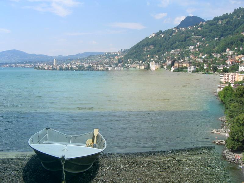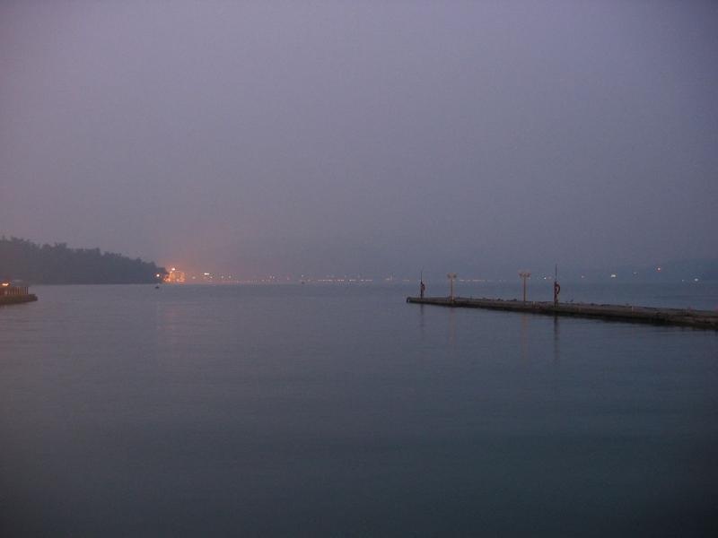
Test Result 2.1

Input Image	Mask

Best-Matching Images	Results

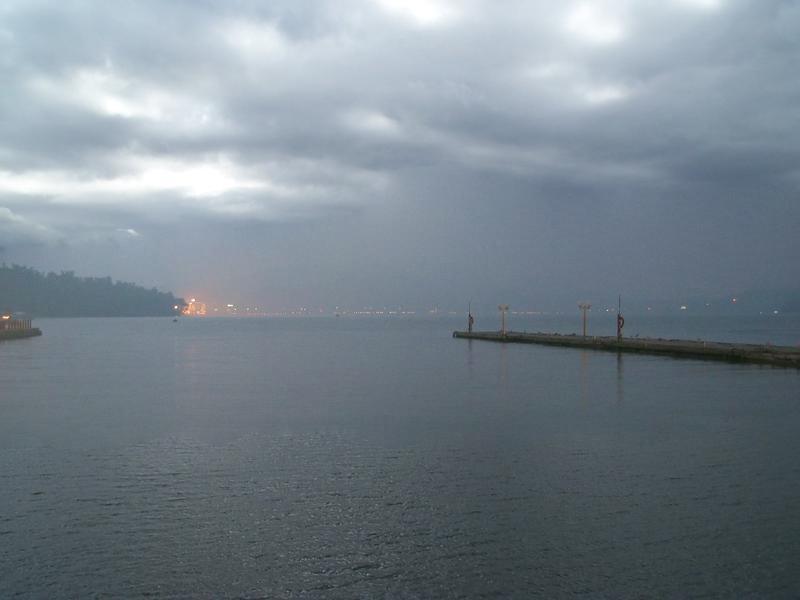
Test Result 2.2

Input Image	Mask

Best-Matching Images	Results

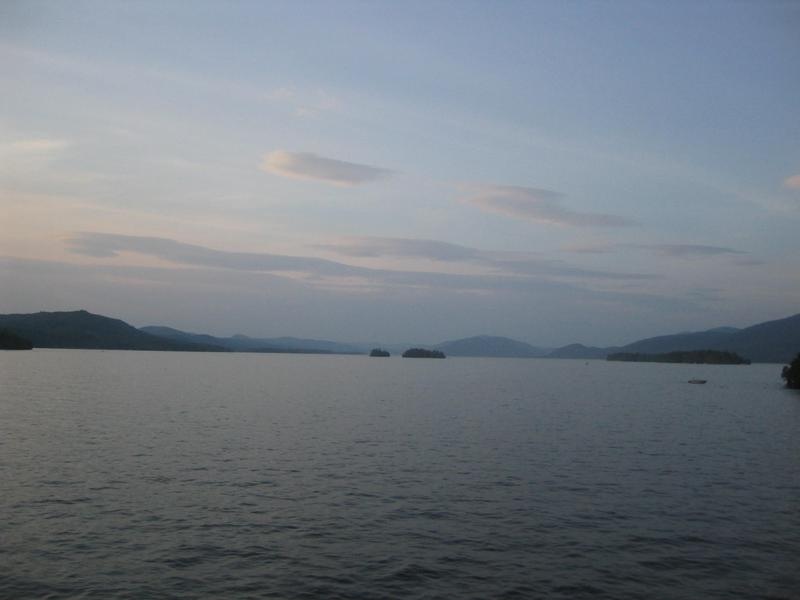
Test Result 3

Input Image	Mask

Best-Matching Images	Results

Reference

James Hays, Alexei A. Efros. Scene Completion Using Millions of Photographs. ACM Transactions on Graphics (SIGGRAPH 2007). August 2007, vol. 26, No. 3.

Oliva, A. & Torralba, A. International Journal of Computer Vision (2001) 42: 145. https://doi.org/10.1023/A:1011139631724

GIST descriptor by tuttieee from Github

Codes from Project 2 and Project 3.