I. Data Collection
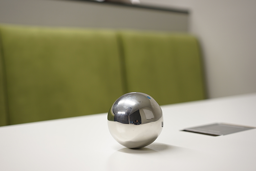
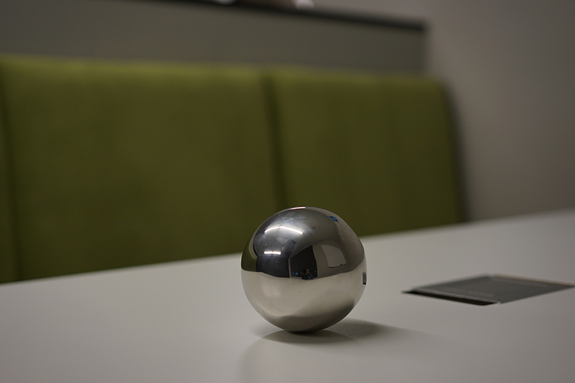
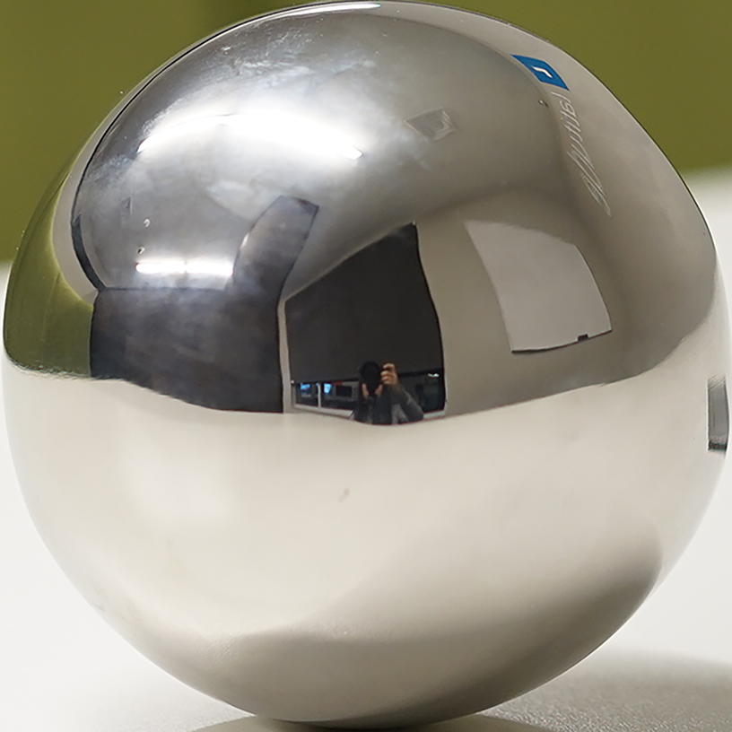
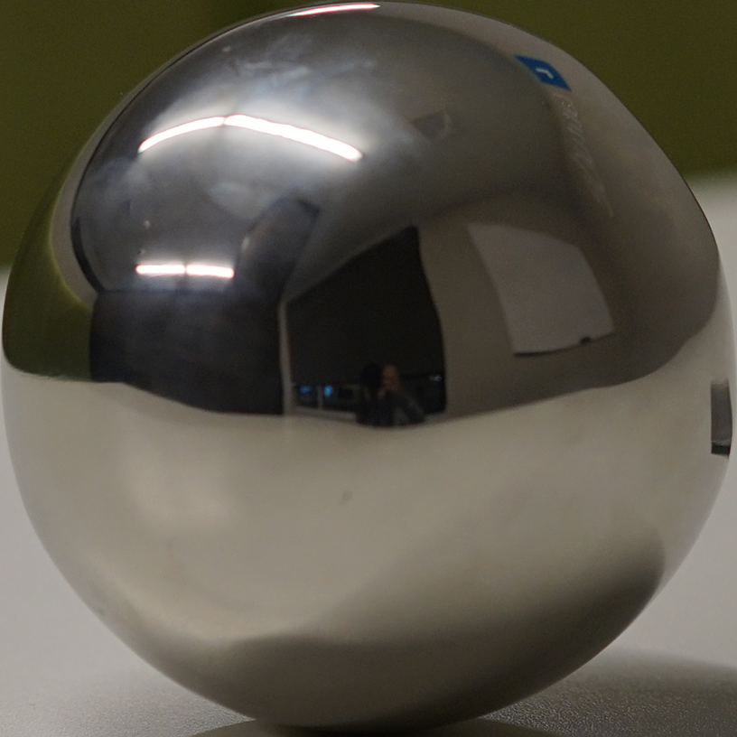
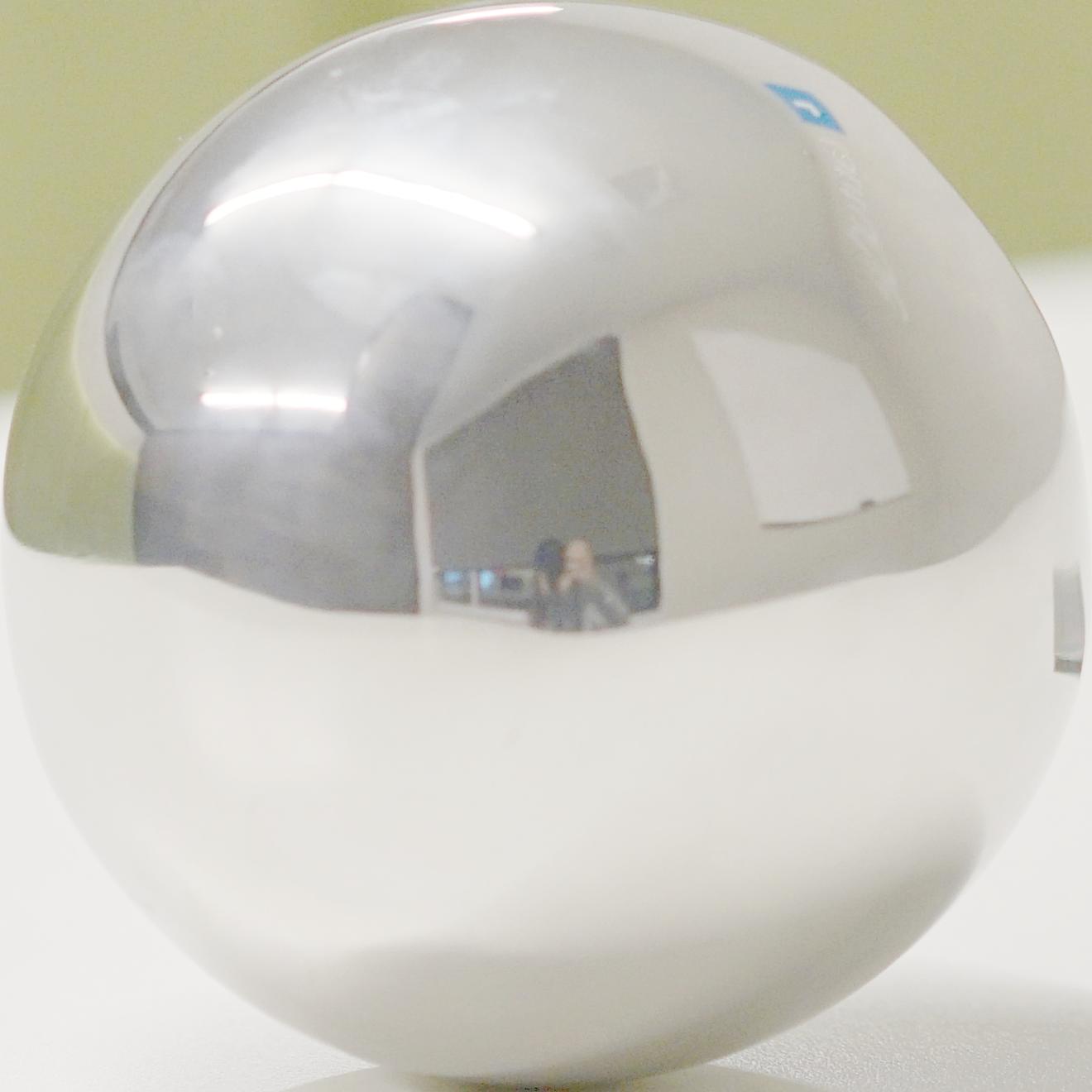
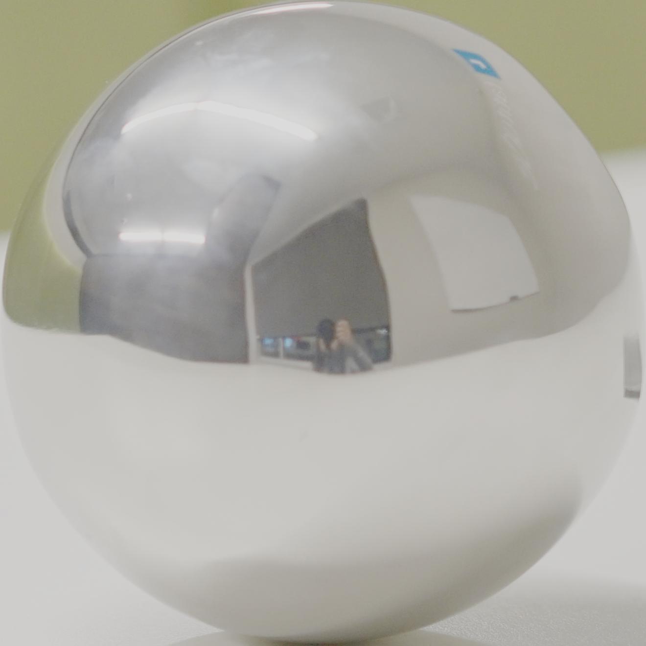
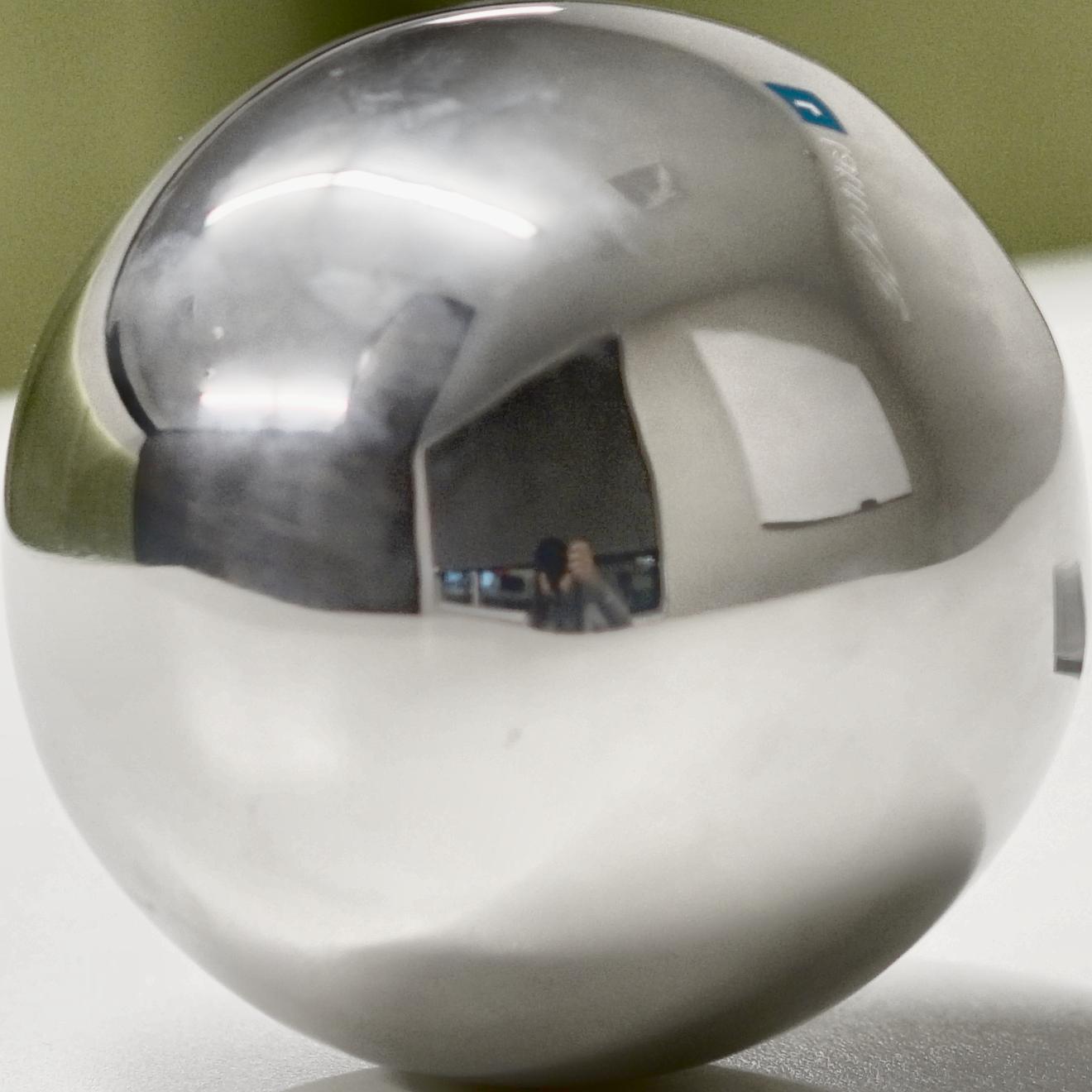
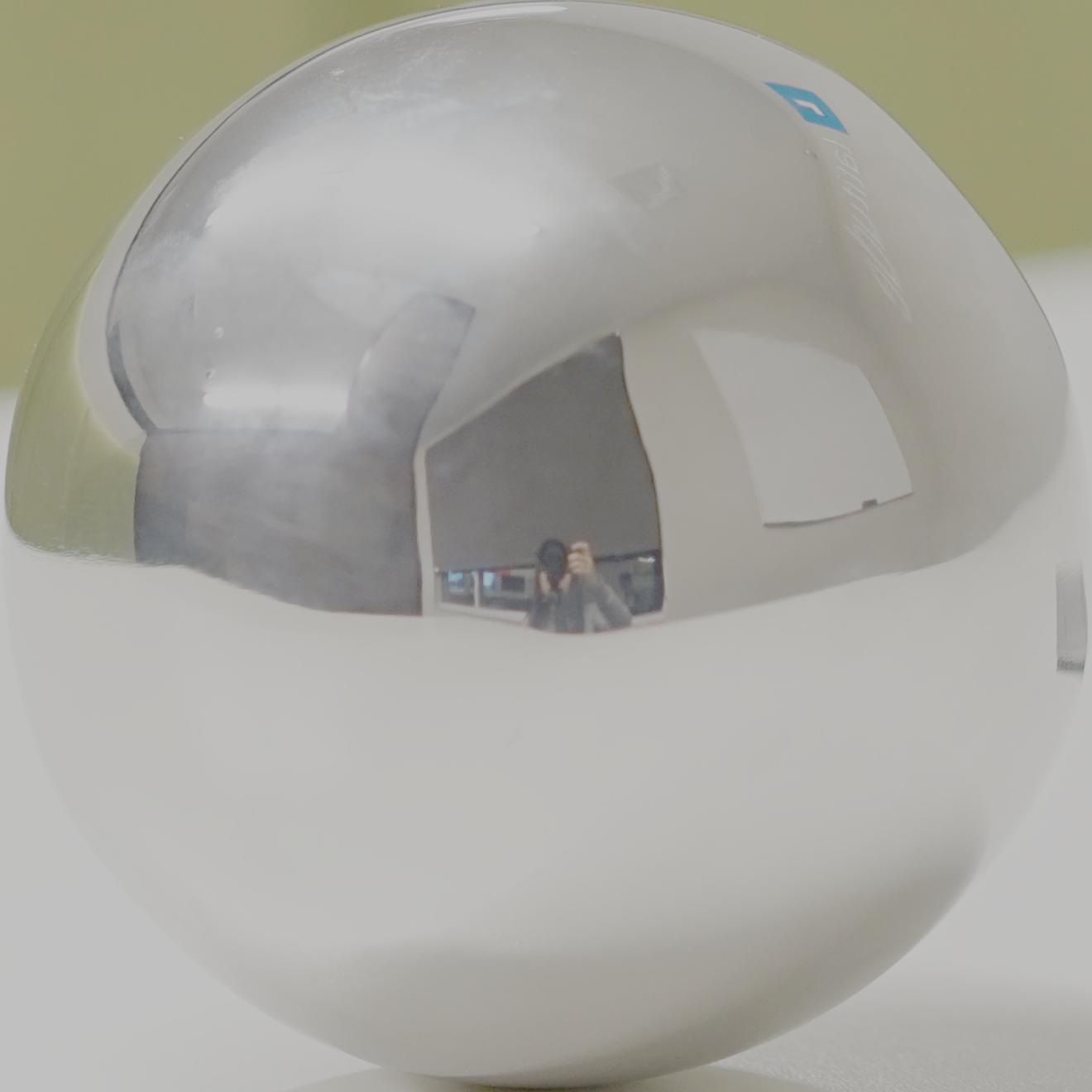
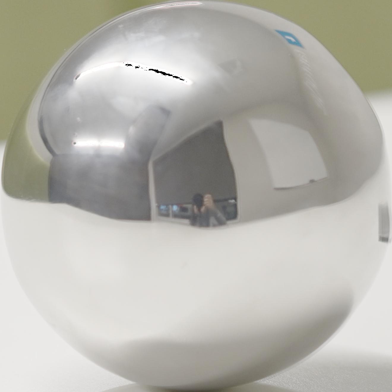
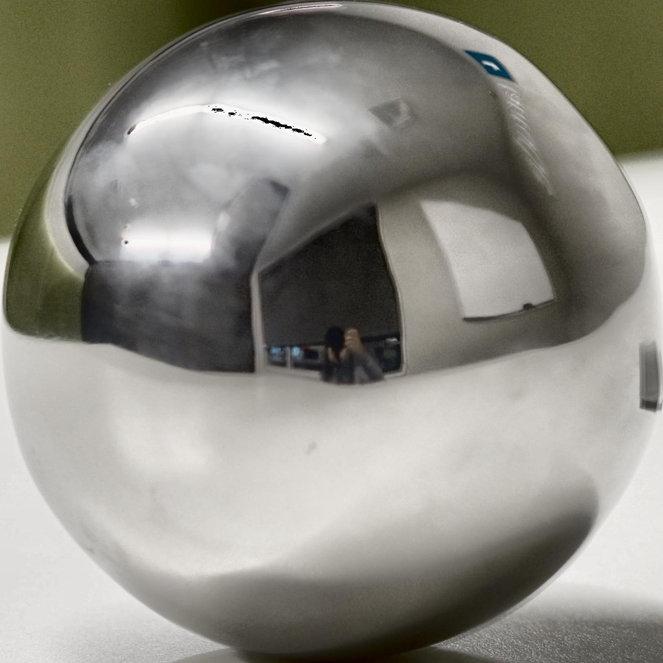
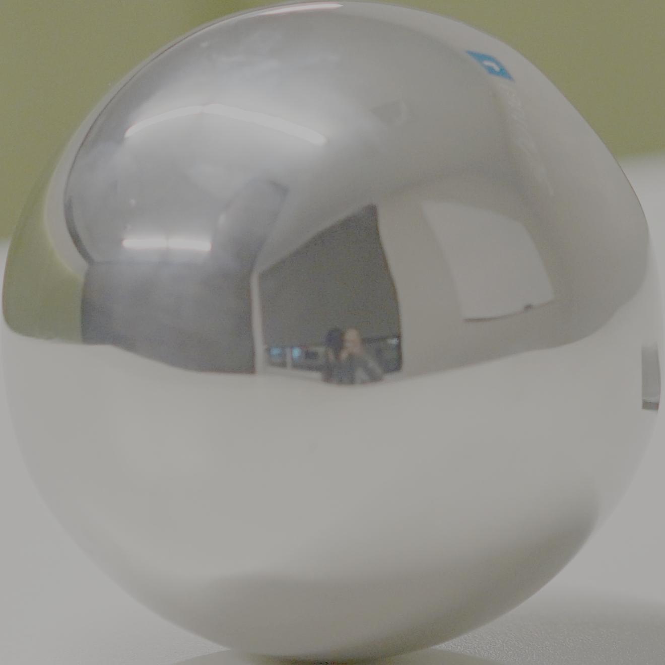
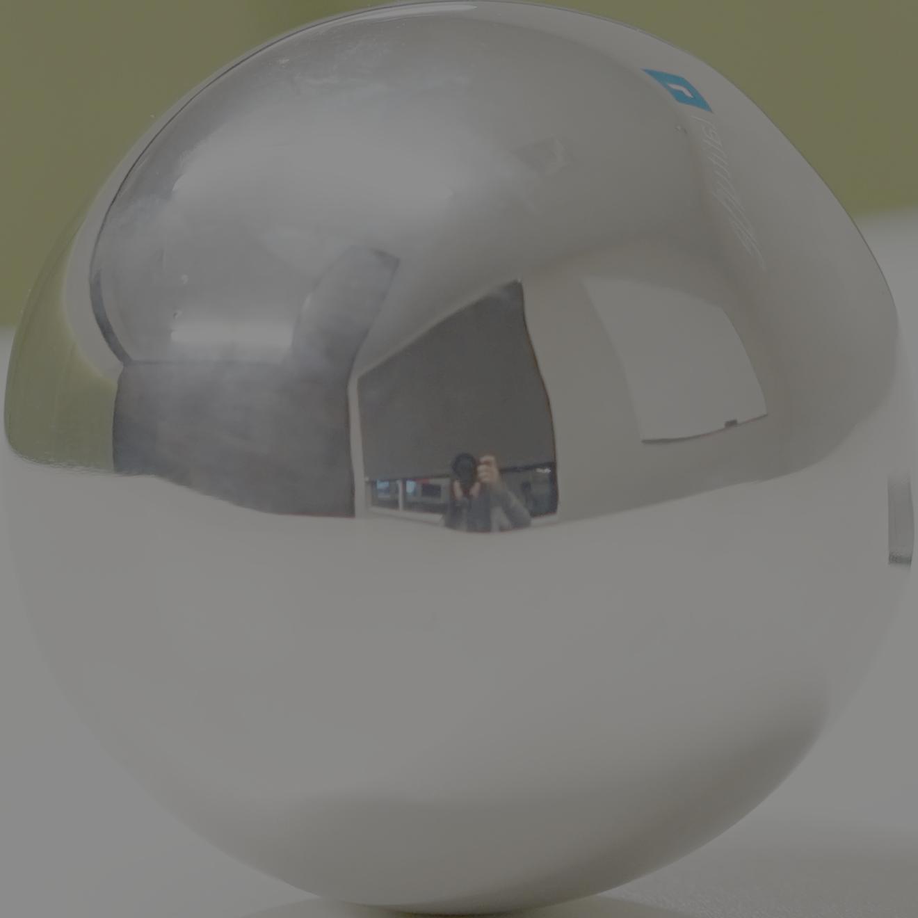
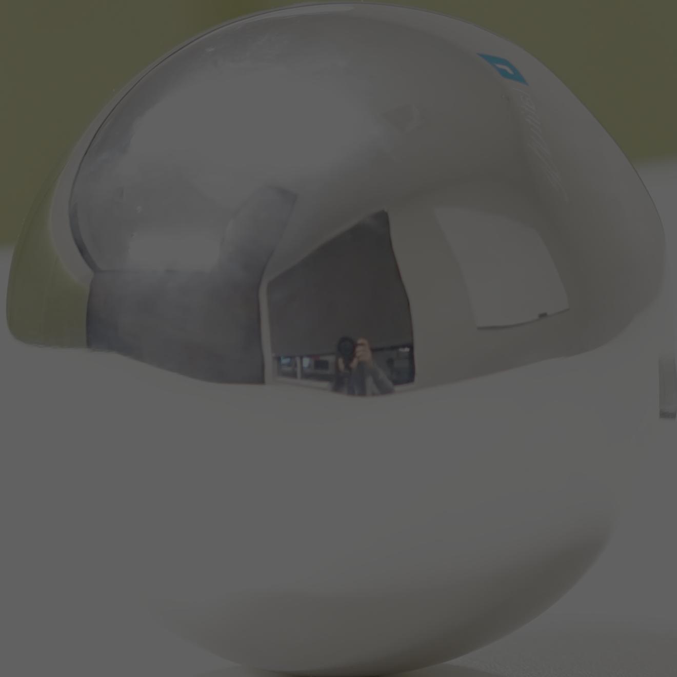
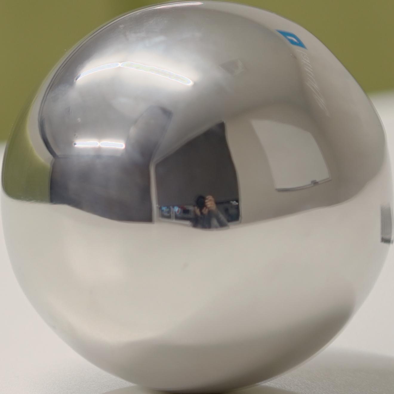
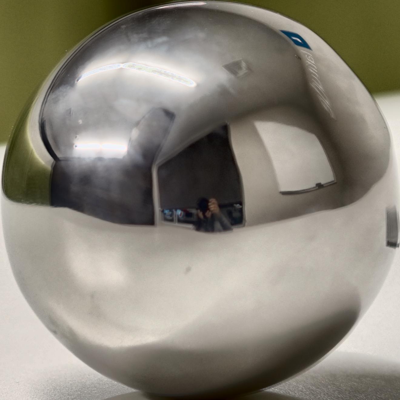
We took three images of the mirror ball in a study room, with different exposure times (1/10s, 1/40s, 1/160s), as well as one image of the empty scene (see part 4).
| 1/10 | 1/40 | /1/160 | |
|---|---|---|---|
| Uncropped | 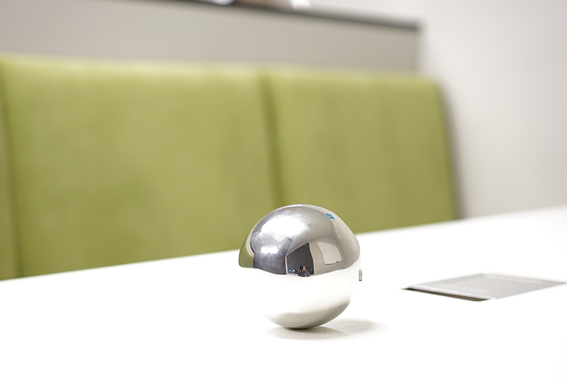 |
 |
 |
| Cropped | 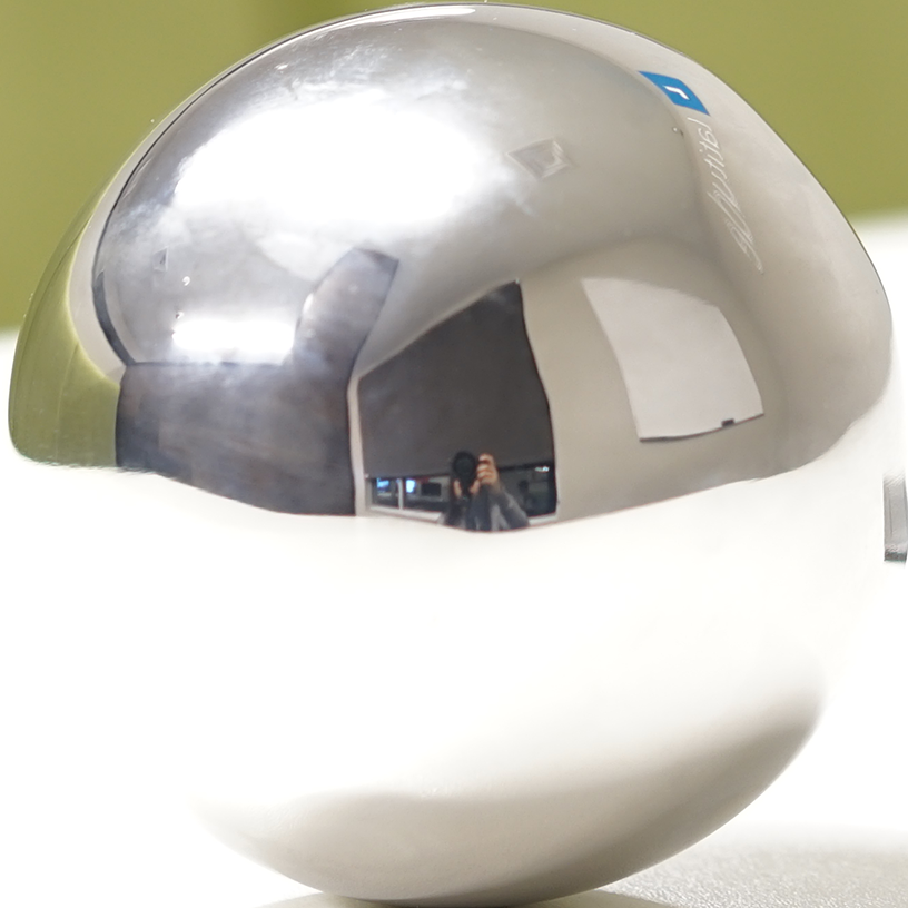 |
 |
 |
II. LDR to HDR
We use three methods to get the HDR images, 1) Naive LDR merging, 2) LDR merging without under- and over-exposed regions, and 3) LDR merging and response function estimation. We include the figures of log irradiance.
Note that we display the images in a smaller scale for better comparison between these stages.
1. HDR Naive
We simply average three scaled LDR images.
| log irradiance of 1/10 | log irradiance of 1/40 | log irradiance of 1/160 | log irradiance | naive hdr |
|---|---|---|---|---|
 |
 |
 |
 |
 |
2. HDR Proper
The idea is to average images after removing under and over exposure pixels. We improve this method by using a weighting function instead, to avoid the case when a given pixel is never properly exposed.
| log irradiance of 1/10 | log irradiance of 1/40 | log irradiance of 1/160 | log irradiance | proper hdr |
|---|---|---|---|---|
 |
 |
 |
 |
 |
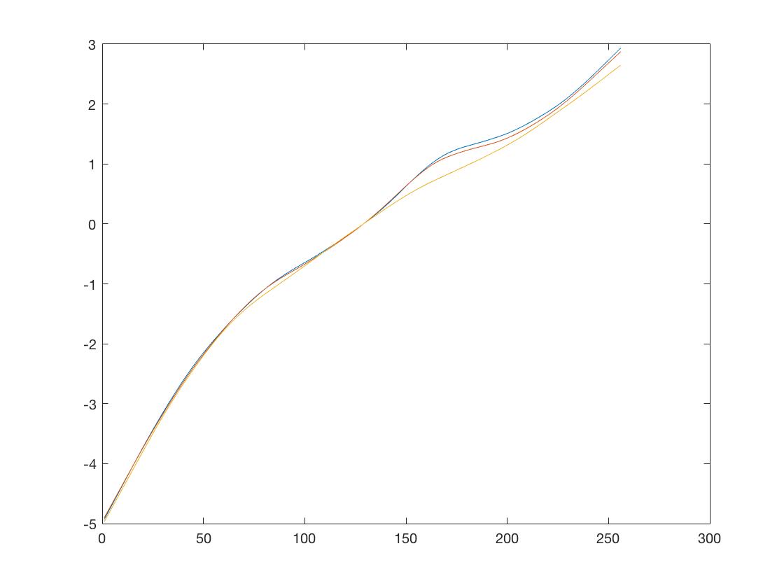
3. HDR Response
This method is based on the formula in Debevec’s paper. We use gsolve to estimate g for each pixel, and recover the HDR image using the given equation.
| log irradiance of 1/10 | log irradiance of 1/40 | log irradiance of 1/160 | log irradiance | response hdr |
|---|---|---|---|---|
 |
 |
 |
 |
 |
Estimate function g:
4. Explanations
We examine log irradiance for three methods, both the source images with different exposure time as well as the results.
For each stage, the irradiances should not be the same even for the sources images. When we calculate the max and min value for scaling, we’ve included the final HDR image, which is different in each stage, so the scaled images, which might be similar with or even equal to each other, are not necessarily identical.
For example, if we choose point (45,56) in Image 1 (1/10s) for each stage, we have (0.7294, 0.7333, 0.5686), (0.7294, 0.7333, 0.5686) and (0.5333, 0.5294, 0.4078). Another examples are point (314,746) in Image 2 (1/40s) for each stage, we have (0.6196, 0.6157, 0.6000), (0.6196, 0.6157, 0.6000) and (0.4471, 0.4431, 0.4275), which is the same for the first two pixels, but different in the third.
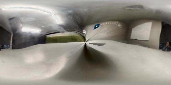
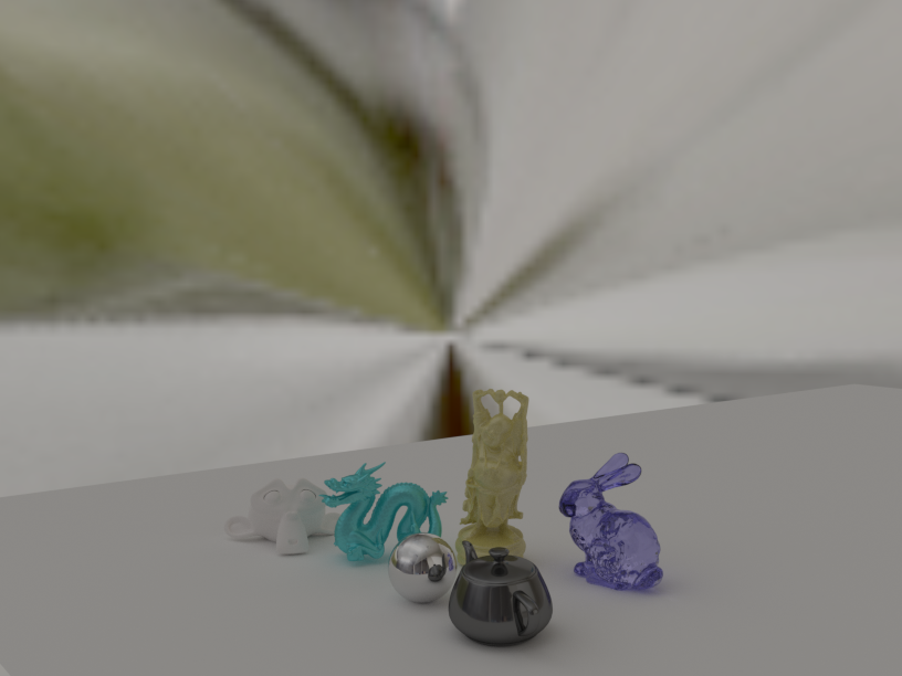
III. Equirectangular Image
Result
Explanation
The transformation, is based on the mapping between the mirrored sphere domain and the equirectangular domain, i.e., by the mapping between phi and theta. We implement this by two steps:</p>
- Sphere domain: We calculate the normals and then the reflection vectors based on the equation
R=V-2.*dot(V,N).*N, and we can get[phis, thetas]pairs from the reflection vectorsR - Equirectangular domain: We obtain the
[phis, thetas]pairs by the formulameshgrid(0:pi/360:2*pi, 0:pi/360:pi)
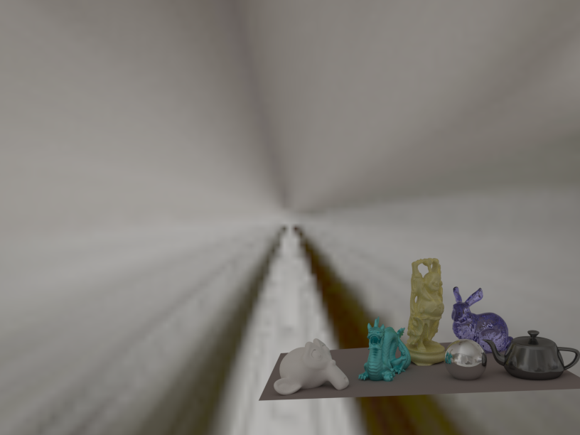
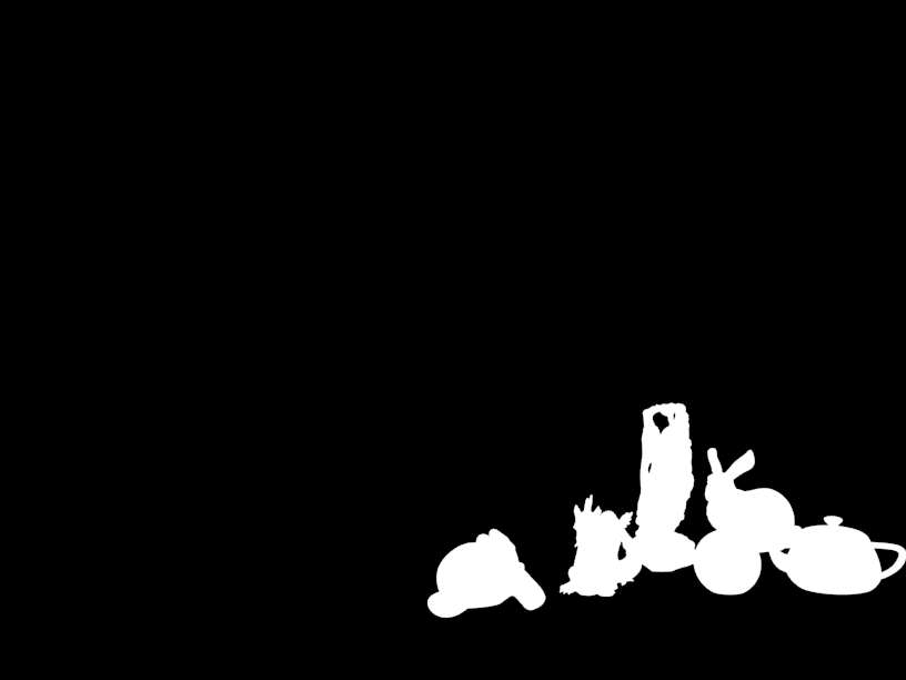
IV. Rendering
We have the empty scene of the study room. We use Blender to render images with and without the objects, and get the mask. Finally we have the composition result.
| Empty scene | Final Result |
|---|---|
 |
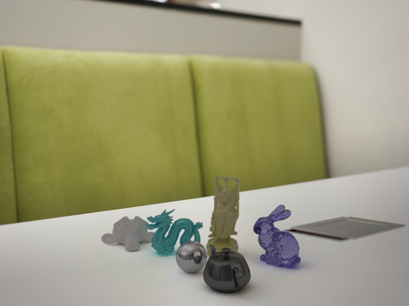 |
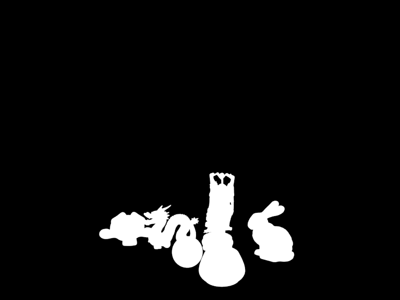
| Rendering without object | Rendering with object | Mask |
|---|---|---|
 |
 |
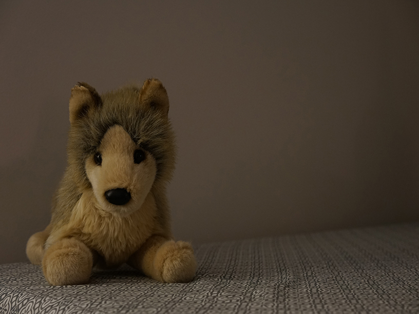
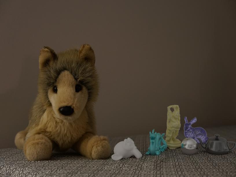
Another example with different scene
Here is another example for a toy on the bed. It is not a good example since we didn’t consider the texture of the sheet. If we look closely to the mirror ball, we will see the plane reflected is plain. Therefore, it would be better if we place the ball on a flat plane, like the example above.
| Empty scene | Final Result |
|---|---|
 |
 |
| Rendering without object | Rendering with object | Mask |
|---|---|---|
 |
 |