Blending
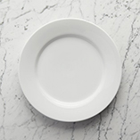
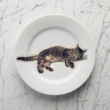
Source and Target Images: I used the cat as the source image and plate as the target image, because the background of the source fits the target quite well.
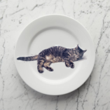
Blended Image: This is the blended image with the source pixels directly copied into the target region. In particular, the shadow of the cat (the left side of its head) doesn’t fit well. After Poisson Blending and Mixed Gradients, the shadow looks better.
Final Blended Image: Specifically, Poisson Blending preserves the source image’s gradient, and also makes sure the border of the source blend in well. Mixed Gradient goes further by using the gradient in source or target with the larger magnitude as the guide, rather than the source gradient.
| Source | Target | Before | Poisson | Mixed |
|---|---|---|---|---|
 |
 |
 |
 |
 |
The biggest question I encoutered is that I didn’t declare A as a sparse matrix, so the whole process is pretty slow.
Two more examples
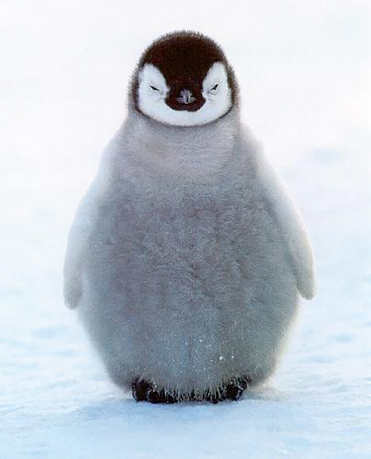
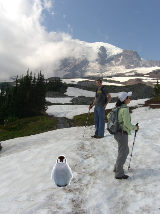
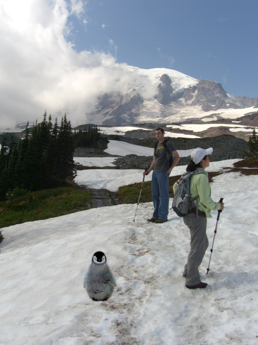
Here are two more examples from the slides, with the original source and target images, as well as the final blending results.
| Source | Target | Before | Poisson | Mixed |
|---|---|---|---|---|
 |
 |
 |
 |
 |
| Source | Target | Before | Poisson | Mixed |
|---|---|---|---|---|
 |
 |
 |
 |
 |
One failed example
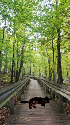
I tried one more cat example, and the cat turned out to be too dark because of the dark color in the background as well as the cat itself.
| Poisson | Mixed |
|---|---|
 |
 |
Implement color2gray.m
I implemented color2gray.m based on the toy problem.
| Color Blind 4 | Color Blind 8 | |
|---|---|---|
| Given original image with digits at the center. |  |
 |
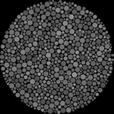
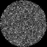
If we change RGB to gray directly using the MATLAB built-in function rgb2gray, the digits are gone because rgb2gray doesn’t preserve the gradient. |
 |
 |
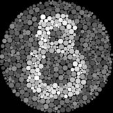
| Using poisson blending, we preserve the gradient, so the contrast between the digits and background is still obvious. | 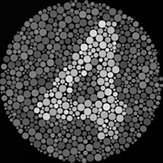 |
 |